In the real world, new conditions and changing scenarios often differ from training data, causing current ML models to fail. Let’s explore this with a hypothetical example.
A self-driving AI’s dilemma
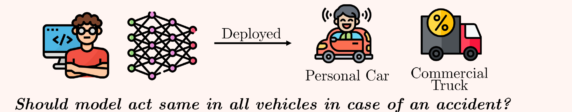
Fig1: A self driving car thought experiment
Consider a self-driving AI trained on data from various countries and driving conditions, now deployed in different vehicles with distinct regulations. Should this AI make the same decision in identical situations across all these vehicles?
The AI must adapt based on the vehicle type. Private cars carry passengers, so the AI should prioritize their safety. In contrast, commercial vehicles carry payloads, and the AI might need to protect humans outside the vehicle in an accident.
Such context-dependent scenarios are common in the real world. Current machine learning models struggle to adapt because developers often “hard-code” notions of generalisation, leading to AI misalignment.
Why AI-Alignment is like gifting?
Imagine this: It’s your best friend’s birthday, and you’ve decided to surprise them with a gift. But there’s a catch — you have no idea what they want. You could buy something random and hope for the best, but chances are, your gift might not hit the mark. This dilemma mirrors a common challenge in machine learning: training models with fixed generalization notions often leads to alignment problems.
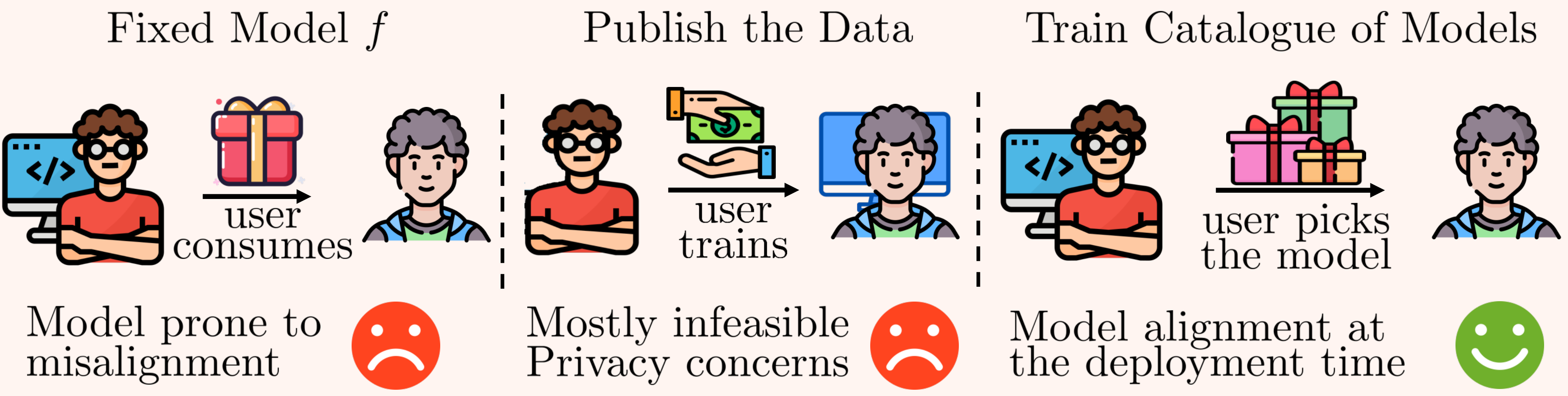
Fig2: We train a bunch of models that the user can pick from at test time.
So, what’s the solution? One might suggest giving users the raw training data to train a model themselves. This is akin to handing over cash instead of a gift, allowing them to get exactly what they want. While this approach ensures alignment, it also places a significant burden on the user and can raise privacy concerns — much like the awkwardness of giving money instead of a thoughtful present.
But what if there was a middle ground? Here’s where our approach comes in. We propose that model developers train a collection of models, each tailored to different potential needs, and then let the user choose the one that best fits their requirements at test time. Think of it as presenting a selection of carefully chosen gifts, allowing your friend to pick the one they love the most. This is what our approach, Imprecise Learning executes!
Sure, this method is more computationally expensive — similar to buying multiple gifts instead of just one. However, it offers the best of both worlds: solving the alignment problem while avoiding the need to release the training data. By providing a range of options, we respect user privacy and make the process more efficient and user-friendly.
How does Imprecise Learning differ ?
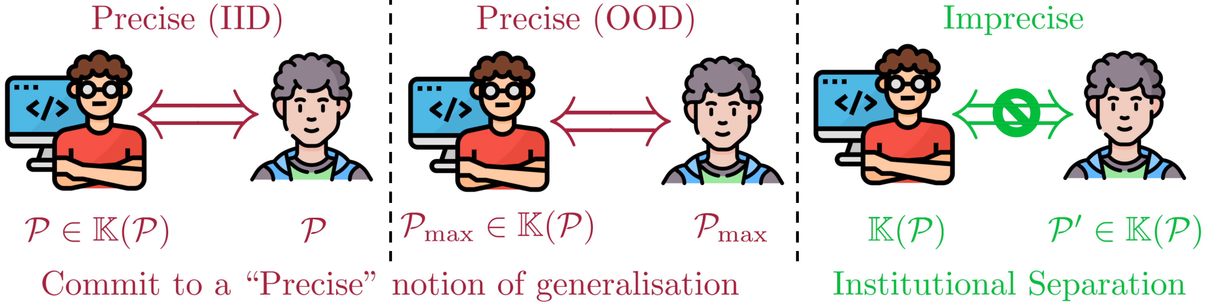
Fig3: How are assumptions different in the Imprecise Learning compared to previous settings.
Generalization is a well-studied topic in machine learning, crucial for understanding the assumptions that ensure learning and how these assumptions play out in real-world scenarios. Broadly, generalization has been explored in two main settings: in-distribution (IID) generalization and out-of-distribution (OOD) generalization. IID settings assume that both training and deployment environments come from an unknown fixed distribution \(\mathcal{P}\). In contrast, OOD generalization relaxes this assumption, allowing for different distributions during training and deployment.
Under the IID assumption, developers know that the test-time distribution matches the training-time distribution, providing a clear understanding of the user’s deployment situation. This allows the learner to optimize precisely for a single distribution. In OOD setting test-time distribution is unknown and the frameworks often optimize for the worst-case distribution, assuming this will cover most scenarios. This approach also represents a precise choice, committing to a specific distribution under uncertainty.
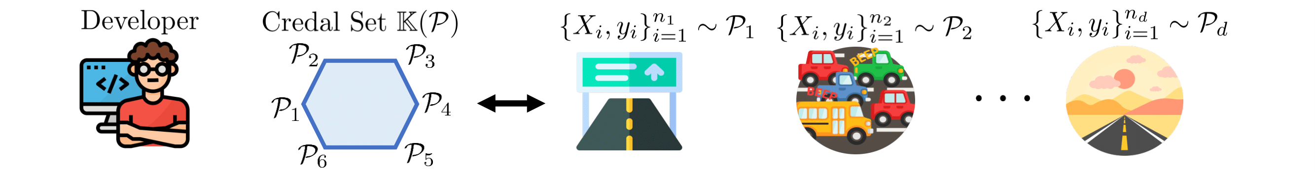
However, precise generalization notions can lead to misalignment due to arbitrary commitments to distributions under uncertainty. Imprecise learning, on the other hand, does not commit to a single distribution. Instead, developers consider a set of possible distributions \(\mathbb{K}(\mathcal{P})\), known as the credal set within the Imprecise Probability community. The credal set represents the set of rational beliefs or distributions that agents can be uncertain about. By acknowledging that developers cannot know all user scenarios and deployment conditions, imprecise learning trains models for various possible distributions within this set.
Imprecise Learning in domain generalisation
To model the concept of imprecise learning, we consider a domain generalization task, a typical OOD problem where learners start with multiple domains \(\{1,\dots,d\}\). For each domain, we define the population risk, which involves three components:
- A Hypothesis class \(\mathcal{F}\)
- A loss function \(\ell\)
- A unknown data generation distribution \(P\)
The population risk is given by:
$$\mathcal{R}(f)=\mathbb{E}_{P}[\ell(f(x),y)]$$
A model that minimizes this risk is called Bayes-optimal:
$$f^*=arg\min_{f\in \mathcal{F}}\mathcal{R}(f)$$
Now in practice when we have data from \(d\) domains we optimize a profile of risks \(\mathbf{\mathcal{R}}=(\mathcal{R_1},\dots,\mathcal{R_d})\). The alignment task involves how we aggregate this risk profile for optimization. A common method is to average the risks:
$$\mathbf{\mathcal{R}}(f)=\frac{1}{d}\sum_{i=1}^d\mathcal{R_i}(f)$$
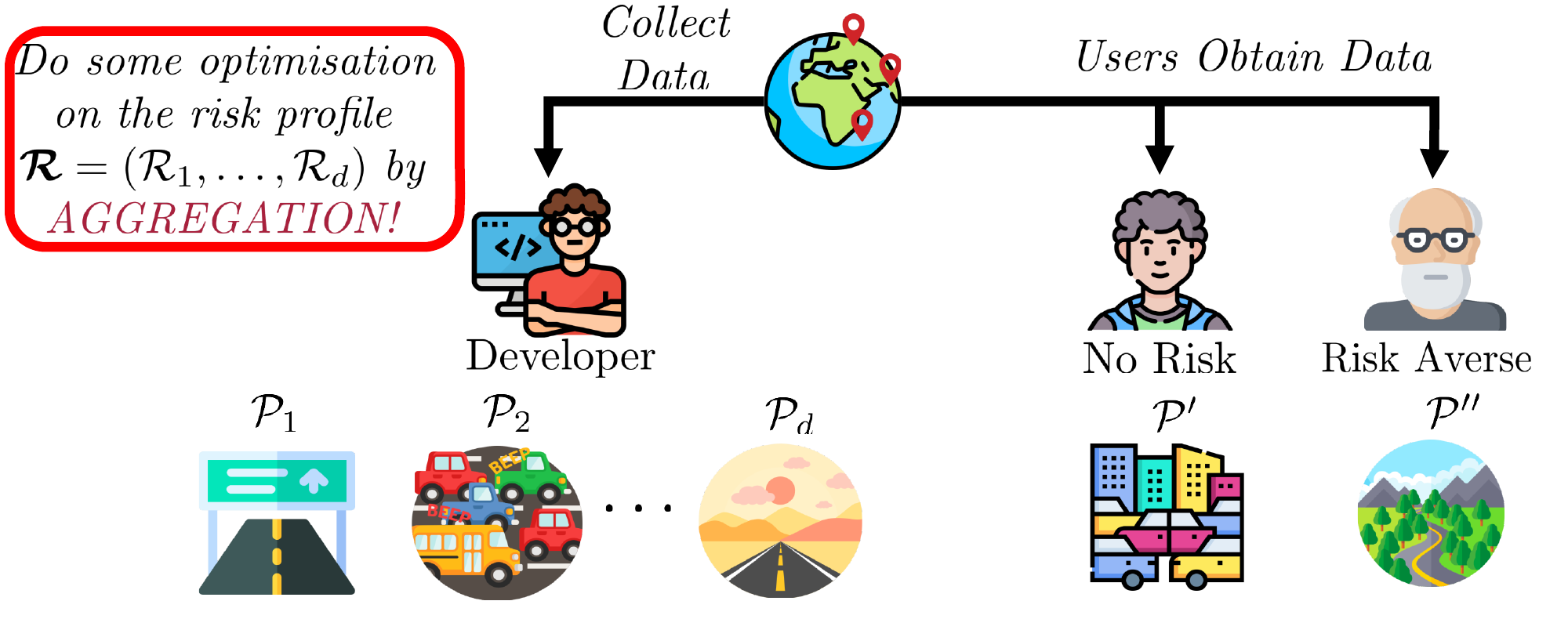
Fig4: How choice of aggerating the risk profile introduces decision making into domain generalisation.
Components of Imprecise Learning framework
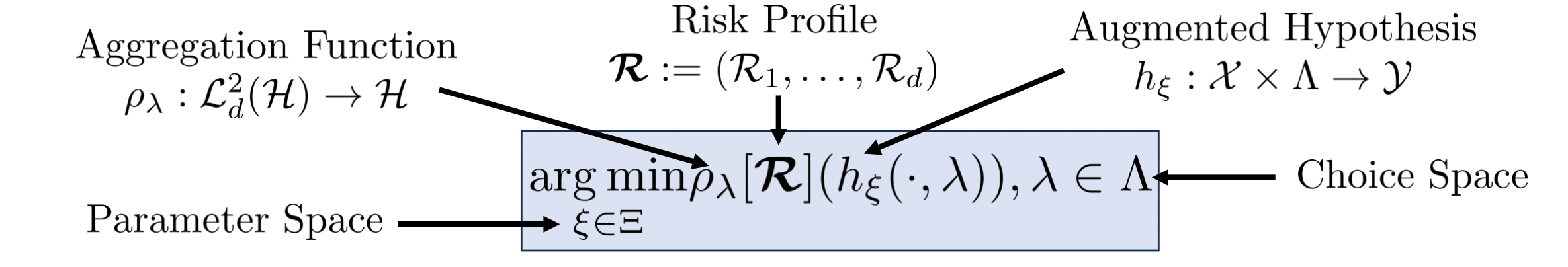
To allow users to decide which notion of generalization the model should follow, we need to create a choice space that enables users to interpret and influence the model’s behavior. We call this choice space \(\Lambda\).
User behavior parameterized objectives
Users choices should influence model behavior. To achieve this, we need to map the \(\lambda\in\Lambda\) to corresponding objective \(\rho_\lambda\). These objectives ensure that the model exhibits user-desired behavior when trained using them.
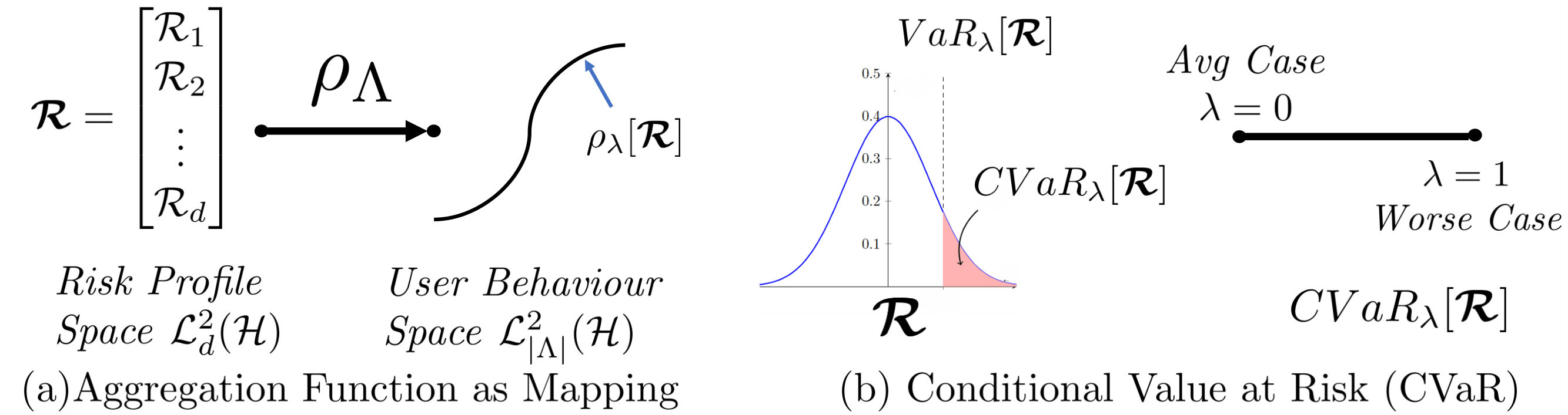
Fig4: Aggregation function allow us to get user behavior parameterized objectives and Conditional Value at Risk (CVaR) is a example of such aggregation.
Augmented Hypothesis
We need to also allow users to recover the model that agrees with their choice at test time, therefore the user’s choice should also influence the model. Therefore, we consider classes of models which depend on both the input and choice for giving output.
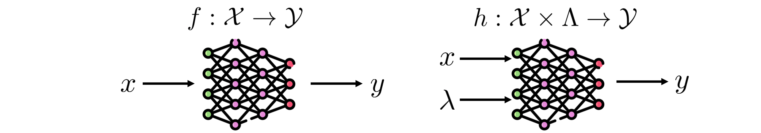
Fig5: Augmented Hypothesis models are user choice dependent.
How do we optimize to learn within such framework?
This section is a bit technical and can be skipped if one is not interested in optimisation. I will try to explain it without going into details of the proofs.
Now that we can characterize user objectives with \(rho_\lambda\) and also find a model trained on it from augmented hypothesis for same \(\lambda\) using \(h(\cdot,\lambda)\) we should try to characterize what Bayes optimality will look like in our setup with an augmented hypothesis \(h\). Naturally, a augmented hypothesis \(h\) can be said Bayes optimal if \(h(\cdot,\lambda)\) is Bayes optimal with respect to every \(\lambda\)
This implies to find an optimal \(h\) we need to solve some multiobjective optimisation problem, however, in our case we can have infinitely many objectives also. So we need to extend the multi-objective optimisation ideas to infinite spectrum of objectives. We solve this problem by marginalising out these infinite objectives with respect to \(\lambda\).
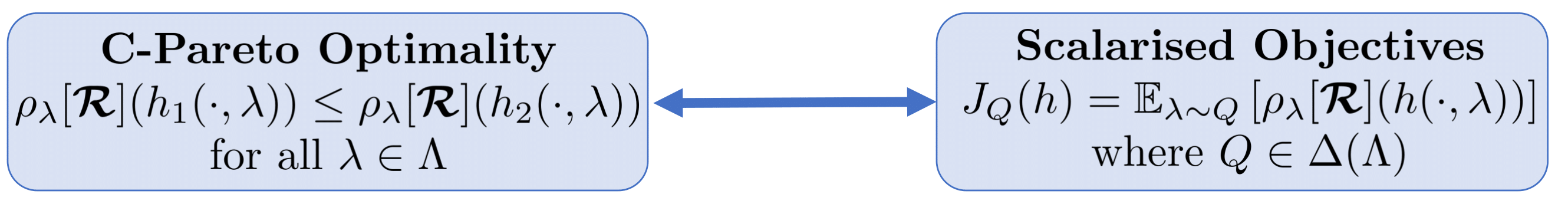
Every choice of distribution \(Q\) corresponds to a point on the Pareto front with respect to objectives \(\rho_\Lambda[\mathbf{\mathcal{R}}]\). However, which \(Q\) can we choose then? We argue that we should choose a \(Q\) that performs Pareto improvement at every update step until Pareto improvements are no longer possible. We explain this with an example
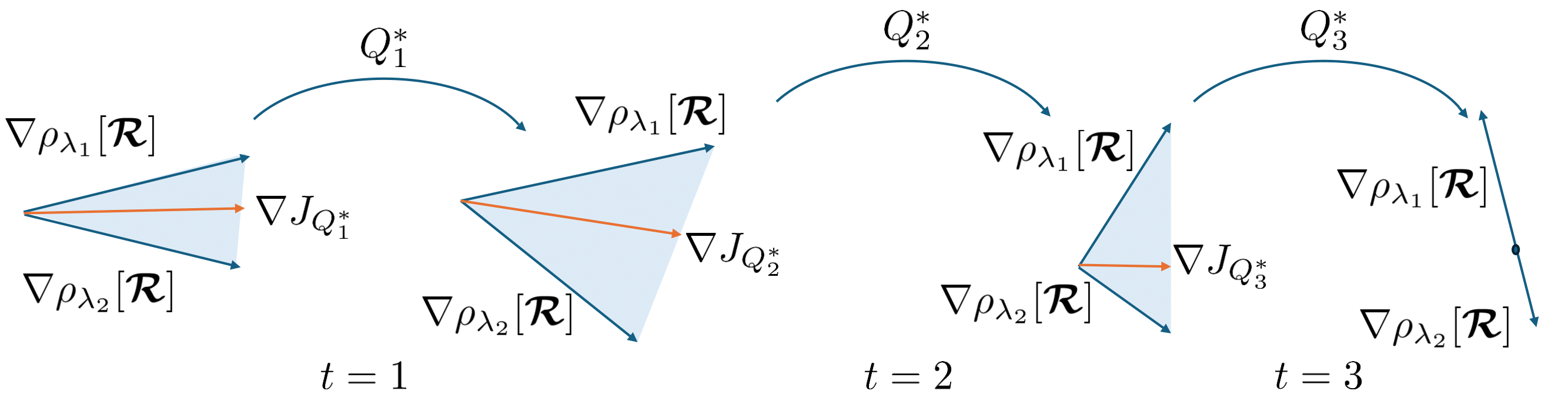
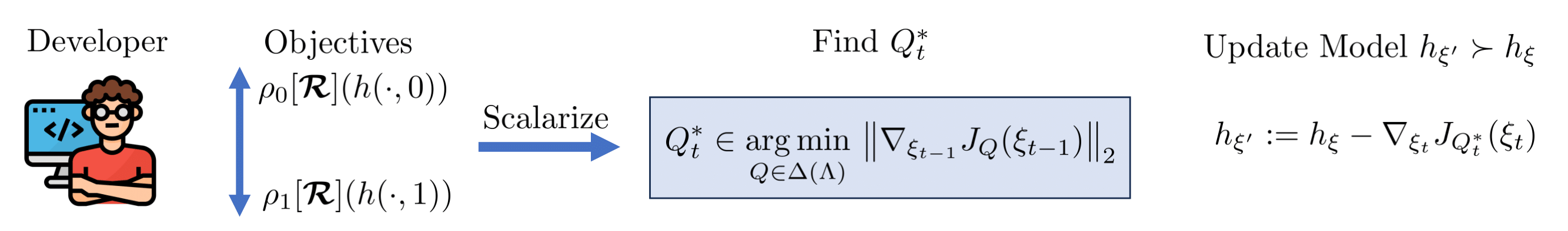
Let’s say we use a fixed distribution \(Q\) for example, uniform. It would work for the first 3 steps but then since \(Q\) is fixed to uniform it will improve the objective 1 at the cost of objective 2 in step 4. We cannot do this since we don’t know yet which objective does the user care about. Therefore we can only make Pareto improvements, which are not guaranteed with a fixed distribution. We find \(Q_t^*\) that guarantees Pareto improvement as follows
$$Q_t^*=arg\min_{Q\in\Delta(\Lambda)}||\nabla \mathbb{E}_{\lambda\sim Q}[\rho_\lambda[\mathbf{\mathcal{R}}](h(\cdot, \lambda))]||$$
Summary
Step 1: Developer represents their uncertainty with credal set
Step 2: Map credal set to user behaviour choice space \(\Lambda\) and pick hypothesis class

Step 3: Find a distribution that makes Pareto Improvement for model update
Step 4: At deployment users can consume model \(h(\cdot,\lambda)\) with their choice of \(\lambda\in\Lambda\)
To learn further about our research you can read our ICML 2024 paper or have a chat with me or my colleagues at the Rational Intelligence Lab who made it possible, Siu Lun Chau, Shahine Bouabid and Krikamol Muandet